
Antenna Range Measurement
In order to practically measure the field strength from an antenna over its entire sphere of radiation, a reference measurement antenna must appear to hover above all the spherical coordinates of the AUT (Antenna Under Test). This can be achieved many ways, but this paper will detail one specific case.The reference measurement antenna will remain fixed and will probe both H and V polarisations.
The AUT will be mounted on a turntable within a turntable. This will allow the antenna to rotate +/- 90 Degrees in the XZ plane (inclination φ) and a full 360 Degrees in the XY plane (rotation θ)
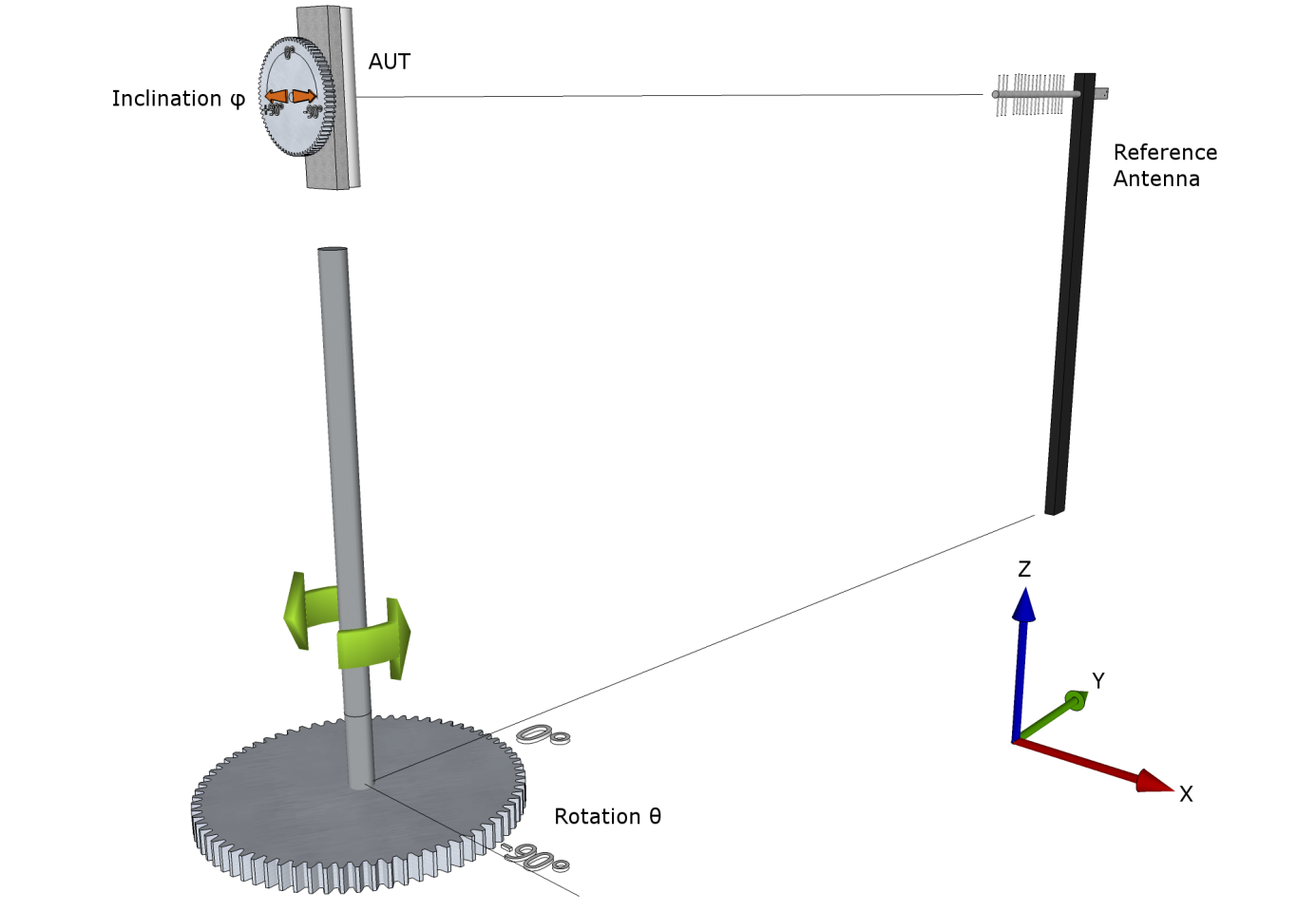
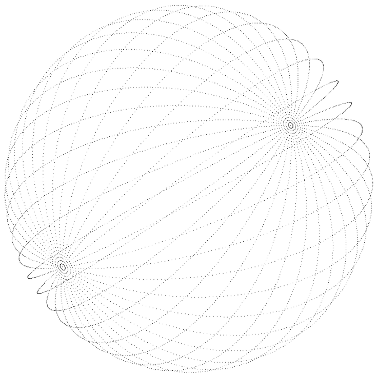
For every setting of Inclination, the will be a full sweep of rotation. A typical scenario would be -90 to +90 in 10 Degree steps of inclination (19 Slices) each with a full rotation of 360 Degrees in 1 degree steps (361 measurements). The total number of data points would be 19*361 = 6859. Here is a representation of all of the measurement points on the sphere scaled to a unit circle.
A more common representation for easy analysis and 3D radiation pattern plotting uses spherical coordinates. We must convert this special case of inclination and rotation to true azimuth-elevation spherical coordinates and this can be achieved using the following formulae.
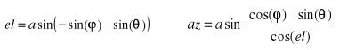
Furthermore, to account for the fact the asin( ) will produce only +/- 90 degrees of azimuth, a correction must be applied to achieve coverage of the rear hemisphere. Simply:
If (rotation > +90°) az = +180° – az
If (rotation < -90°) az = -180° – az
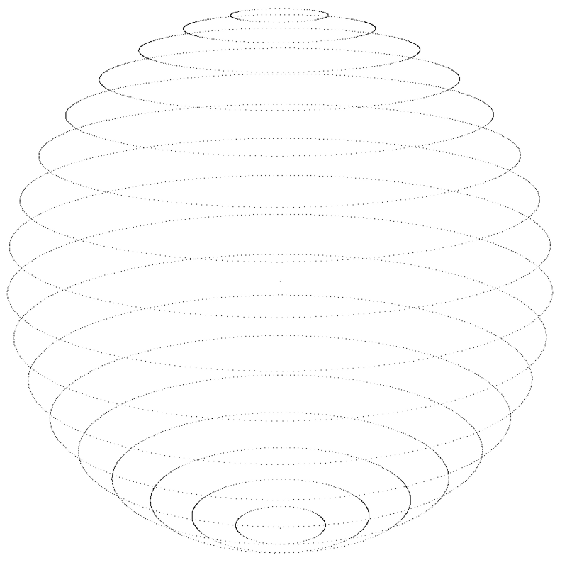
The next Figure shows how the unit sphere is covered by azimuth- elevation coordinates.
Each azimuth ring in the figure is at a different elevation ranging from -90° to +90°.
The antenna is not actually measured this way as it becomes obvious that less sphere coverage is achieved due to there being a greater concentration of points at the poles.
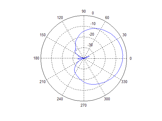
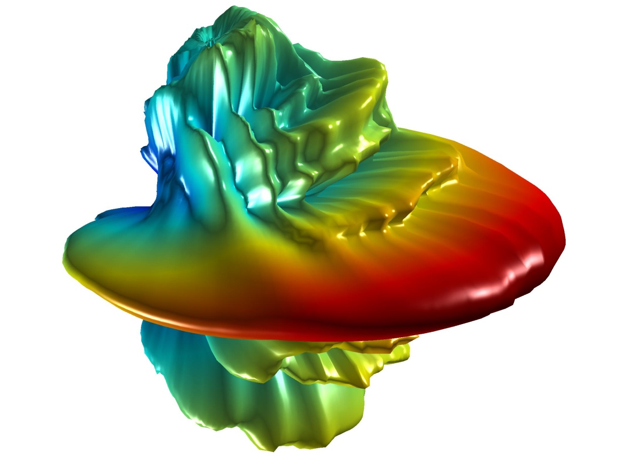
Example Azimuth, Elevation and 3D plots (4 element antenna)
These plots demonstrate the output from the described procedure. They were drawn using MATLAB which was also used to perform the coordinate conversion.
Elevation slice (az = 0°)

Azimuth Slice (el = 0°)
3D pattern.
MATLAB Code
%Import the file: Antenna range uses the following
%representation: rotation -90 to +90 and az -180 to 180
DELIMITER = ' ';
HEADERLINES = 1;
A = importdata('D:\Data\antenna.dat', DELIMITER, HEADERLINES);
%Create new variables in the base workspace from those fields.
rot = A.data(:,1);
dE = A.data(:,2);
dH = A.data(:,4);
%Choose the data to plot. In this case sum both polarisations for full
%copolar field
r = 10 .* log10((10.^(dE ./ 10 )) + (10 .^ (dH ./ 10 )));
%Scale to zero if not already
rmax = max(r);
r = r - rmax;
%Create rotational data as this table is not explicitly in the file
z = ones(361,1);
z = z * -90;
inc = [z;z+10;z+20;z+30;z+40;z+50;z+60;z+70;z+80;z+90;z+100;z+110;z+120;z+130;z+140;z+150;z+160;z+170;z+180];
%Convert all to radians
inc = inc * pi/180;
rot = rot * pi/180;
%Calculate the elevation from the rotation and azimuth
el = asin(-sin(inc) .* sin(rot));
%Calculate the azimuth from the inclination and rotation and elevation
%Ensure inverse sin doesn't see greater than 1 due to bad rounding
az = asin( cos(inc) .* sin(rot) ./ (cos(el) + 0.0000000001) );
%Correct for quadrant of azimuth lost by the inverse sin
form = 1:6859
ifrot(m) > (pi/2)
az(m) = pi - az(m);
elseifrot(m) < (-pi/2)
az(m) = - pi - az(m);
end
end
%Scale so as to remove the negative numbers not tolerated by surface.
%Also remove any detail less than -40dB to aid visibility
r = r + 40;
form = 1:6859
if r(m) < 0
r(m) = 0;
end
end
%Polar Elevation plot from 0 to -40dB
figure('Position',[700 200 400 400]);
set(gcf,'Name','Elevation Slice','NumberTitle','off');
polar(rot(1:361)',r(1:361)','-r');
%Polar Azimuth plot from 0 to -40dB
figure('Position',[700 700 400 400]);
set(gcf,'Name','Azimuth Slice','NumberTitle','off');
polar(rot(3250:3610)',r(3250:3610)','-r');
%3D Plot initialisation
MOVFIG = figure('Position',[20 600 640 480]);
set(gcf,'Name','3D Polar plot','NumberTitle','off');
%Develop a uniform grid in 2 degree steps for az and el
azs = -180*pi/180;
azi = 2*pi/180;
aze = 180*pi/180;
els = -90*pi/180;
eli = 2*pi/180;
ele = 90*pi/180;
[Az_m El_m] = meshgrid(azs:azi:aze,els:eli:ele);
%Interpolate the nonuniform gain data onto the uniform grid
Zi = griddata(az,el,r,Az_m,El_m,'cubic');
%Generate the cartesian coordinates
[x y z] = sph2cart(Az_m,El_m,Zi);
%Plot surface and colour according to Zi
surf(x,y,z,Zi)
%colourmap and colorbar
colormap(jet(1024));
%c_vect = [0 40];
%caxis(c_vect);
%colorbar
%OpenGL renderer lighting and shading
set(gcf,'renderer','OpenGL', 'resize','off');
lighting phong
shading interp
set(gcf,'color',[0.6 0.6 0.6]);
%Light Source 1 and 2
g = light;
p = light;
set(g,'Style','infinite', 'position',[1 1 1]);
set(p,'Style','infinite', 'position',[-1 -1 -1]);
%Other items
material shiny
axis off vis3d
box off
view([45,0])
drawnow
%Create movie if you wish
nFrames = 180;
mov(1:nFrames) = struct('cdata',[], 'colormap',[]);
fork = 1:nFrames
view([k*2,0])
mov(k) = getframe(gcf);
end
movie2avi(mov, 'Ant_movie2.avi', 'compression', 'none', 'fps',30, 'colormap', 'jet');